Each merchant in our system has the following characteristics:
Merchant location
Merchant serviceability distance (i.e. places where the merchant delivers)
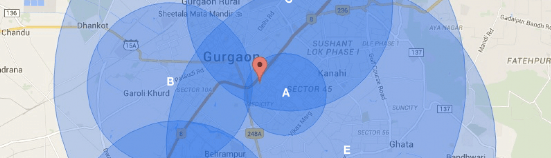
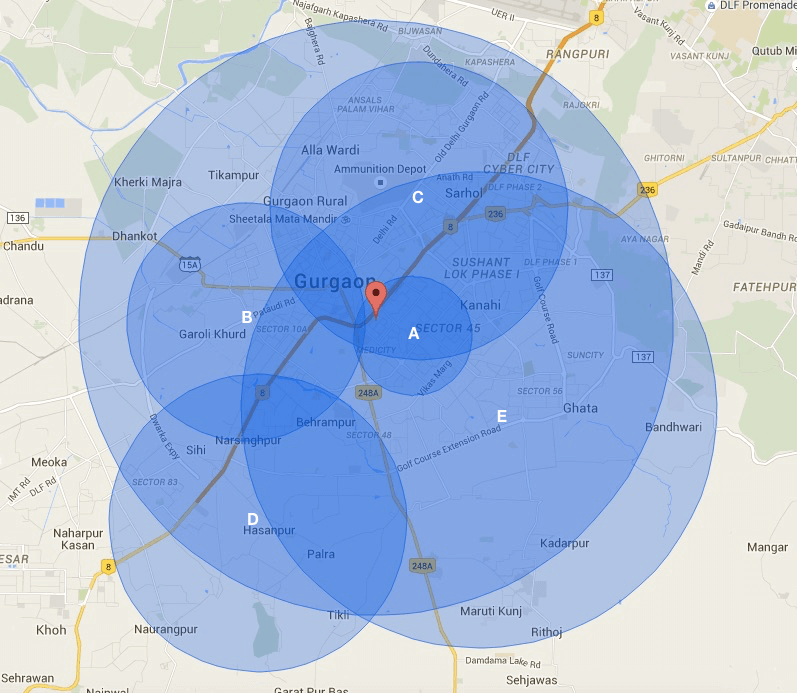
As soon as the user opens the consumer app, the user location gets fired. We consider a list of potential merchants which fall in the circular area centred around the user location. Each merchant has his own serviceability area centred around his/her location. The intersection of these areas gives us the list of visible merchants. As shown in the above figure, there are 5 merchants in the vicinity of the customer. But only, A, C, and E are visible to the customer.
The present system is flawed in the following ways:
We use radial distances to make these computations. The actual distance could be much more than the radial distance, hence, the last mile team incurs a loss on mileage
In addition to the serviceability distance, last-mile also has a promise time defined for each merchant. The time that is taken to procure goods from a merchant and transporting it to the customer varies. For example, in the evening and mornings, due to traffic, the time could be more than the promise time. At the same time, in a lean period (non-traffic), the delivery bike or car can cover a greater distance within the same promise time
A very straightforward way to solve the above problem is to use Google Distance Matrix API which provides us with real travel time at a given time of the day taking into account current traffic. But, using the API has its own limitations:
There is a rate limit on the number of API calls we can make to Google
The subscription to these calls is very expensive
There is a limit to the number of source-destination pairs we can query at one time
Iris attempts to do what Google Distance Matrix API lets us do, taking care of all the problems we mentioned above.
How to determine travel time in the setup
To achieve the above, we needed a new way to represent lat/long points. The idea is to hierarchically divide the entire area into a set of different cells (tiles). The goal of this decomposition is
High enough resolution for indexing geographic features
Compact representation of each such tile
Very fast method for querying with arbitrary regions (e.g. containment queries)
The tiles at each resolution should have similar area
This is easily achievable by quad-trees. Quad-trees are excellent data structures to hierarchically divide a region. It is used in a host of computer graphics applications to cull view frustum and to detect collisions.
So, how do we decompose a sphere like earth into a quad-tree?
Quad-tree cell
Pretend that earth is a solid sphere inside a unit cube as shown below:
The cube volume is 1x1x1. Project a point p onto the cube and build a quad-tree on each cube face. Then we find the quad-tree cell that contains the projection of p. So the first step is to map this point to the 3D coordinate system.
Thus,
p = (lat,lng) → (x,y,z)
After that, we project this point p to cube face along a radius as shown below:
The problem here is that same area cells on the cube have different sizes on the sphere. In order to sort this, we do a non-linear transformation as shown below:
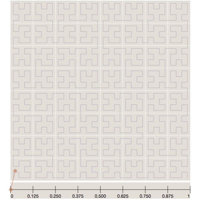
The pink area is a leaf cell, at the bottom of the tree. After this space is discretized, the cells are enumerated on a Hilbert Curve. Hilbert curve is a space-filling curve that converts multiple dimensions into one dimension that has a special feature: it preserves the spatial locality.
First 8-steps towards building a Hilbert Curve (Image source: Wikipedia)
The Hilbert curve is a space-filling curve, which means that its range covers the entire n-dimensional space. To understand how this works, you can imagine a long string that is arranged on the space in a special way such that the string passes through each square of the space, thus filling the entire space. To convert a 2D point along to the Hilbert curve, you just need to select the point on the string where the point is located. This iterative example illustrates this point. It shows the correspondence between the 2D-point and the corresponding point on the curve. In the image below, the point at the very beginning of the Hilbert curve (the string) is located also at the very beginning of curve (the curve is represented by a long string in the bottom of the image):
Correspondence between a 2-D point and Hilbert Curve
Now in the image below where we have more points, it is easy to see how the Hilbert curve is preserving the spatial locality. You can note that points closer to each other in the curve (in the 1D representation, the line in the bottom) are also closer in the 2D dimensional space (in the x,y plane). However, note that the opposite isn’t quite true because you can have 2D points that are close to each other in the x,y plane that are not close in the Hilbert curve.
2-D points close to each other are not close to each other in the corresponding hilbert curve
We will use Hilbert Curve to enumerate the cells. This essentially means that cell values close in value are also spatially close to each other. When this idea is combined with the hierarchical decomposition, you have a very fast framework for indexing and for query operations.
Cell representation
We will enumerate cells along a Hilbert space-filling curve. It is very fast to encode and decode (bit-flipping) and it preserves spatial locality.
The above figures show the cell id representation schema. The first one is representing a leaf cell, a cell with the minimum area usually used to represent points. As you can see, the 3 initial bits are reserved to store the face of the cube where the point of the sphere was projected, then it is followed by the position of the cell in the Hilbert curve always followed by a “1” bit that is a marker that will identify the level of the cell. So, to check the level of the cell, all that is required is to check where the last “1” bit is located in the cell representation. The checking of containment, to verify if a cell is contained in another cell, all you just have to do is to do a prefix comparison. These operations are really fast and they are possible only due to the Hilbert Curve enumeration and the hierarchical decomposition method used.
Using the above representation, every square cm of the earth can be presented using a 64-bit integer.
Representing a covered region
Once we have figured out the cell representation, we can represent a closed polygon as a set of these cell-Ids. In the above figure, we can see Delhi being represented as a set of cells. Each cell area varies from 70 square meters to 310 square meters.
Implementation
Once we have the representation of each city as defined above, we list down all the merchants in these cells. Then, we take the centre of each if these merchants containing cell and populate the adjacent cells for visibility. We pre-populate the visible cells using initial seed data collected from our deliverer app and store it in a cache. So each entry in the cache would have a key as cellId and value as a set of visible merchants from this particular location. We repeat this exercise for each time of the day.
Now, whenever a user opens up his/her app, we find the corresponding cellId for the location, check the cache for this key, and return the set of merchants visible. Since each request is processed via the cache, it is very fast. Please note that no computation happens in real time. Moreover, the system is written using reactive programming techniques. As a result, we achieve high scalability (both vertical and horizontal), complete non-blocking IO and resiliency.
In 1981, Xerox PARC introduced the first Graphical User Interface (GUI), marking a significant shift in computing. Over 43 years, rounded corners have evolved from a design embellishment to an industry standard in both software and hardware.
Setting up our printout delivery store has been extremely satisfying at many levels. At one end is the joy from customers discovering an easy, home-delivered solution for last-minute printouts.
In today’s world, given the pace at which data operates, we need a tool that can help us to generate reports faster and bring out insights within milliseconds.